Analysis of 10x Visium mouse brain slice#

In this tutorial, we demonstrate SpaSRL on the analysis of 10x Visium Mouse Brain Serial Section 1 (Sagittal-Anterior) slice including

Self-representation learning
Spatial domain identification
Spatial domain annotation
Finding differentially expressed genes

The dataset is available at 10x genomics website (Spatial Gene Expression >> Visium Demonstration (v1 Chemistry) >> Space Ranger 1.0.0 >> Mouse Brain Serial Section 1 (Sagittal-Anterior)).

[1]:

import numpy as np
import pandas as pd
import scanpy as sc
import matplotlib.pyplot as plt
import SpaSRL

%matplotlib inline

Data loading and preprocessing#

We load the dataset and perform preprocessing including finding highly variable genes and log transformation.

[2]:

adata = sc.read_visium('./data/Mouse Brain Serial Section 1 (Sagittal-Anterior)/')
adata.var_names_make_unique()
adata

Variable names are not unique. To make them unique, call `.var_names_make_unique`.
Variable names are not unique. To make them unique, call `.var_names_make_unique`.

[2]:

AnnData object with n_obs × n_vars = 2696 × 31053
    obs: 'in_tissue', 'array_row', 'array_col'
    var: 'gene_ids', 'feature_types', 'genome'
    uns: 'spatial'
    obsm: 'spatial'

[3]:

sc.pp.highly_variable_genes(adata, n_top_genes=2000, flavor='seurat_v3')
sc.pp.log1p(adata)

Self-representation learning#

We select landmark samples and then use selected landmarks to run self-representation learning.

[4]:

SpaSRL.select_landmarks(adata, n_landmarks=1000)

 84%|████████████████████████████████████████████▎        | 1670/2000 [00:54<00:10, 30.42it/s, seleted landmarks: 1000]

[5]:

SpaSRL.run_SRL(adata, Lambda=0.1, n_neighbors=200)

 21%|██████▍                       | 107/500 [00:02<00:07, 52.68it/s, relChg: 2.714e-05, recErr: 9.931e-06, converged!]

This is how the adata looks like after self-representation learning.

[6]:

adata

[6]:

AnnData object with n_obs × n_vars = 2696 × 31053
    obs: 'in_tissue', 'array_row', 'array_col', 'is_landmark'
    var: 'gene_ids', 'feature_types', 'genome', 'highly_variable', 'highly_variable_rank', 'means', 'variances', 'variances_norm'
    uns: 'spatial', 'hvg', 'log1p', 'select_landmarks', 'representation'
    obsm: 'spatial'
    obsp: 'representation'

Spatial domain identification#

We identify spatial domains using the representation matrix.

[7]:

sc.tl.leiden(adata, resolution=2.6, neighbors_key='representation')

[8]:

sc.pp.pca(adata)
sc.tl.umap(adata, init_pos='random', neighbors_key='representation')

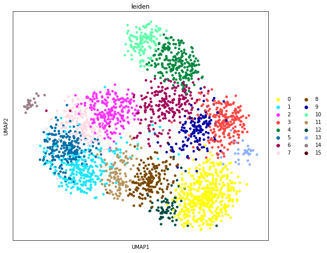
We visualize the inferred spatial domains in UMAP space.

[9]:

fig, axs = plt.subplots(figsize=(9, 7))

sc.pl.umap(
    adata,
    color="leiden",
    size=100,
    palette=sc.pl.palettes.default_102,
    legend_loc='right margin',
    show=False,
    ax=axs,
)

plt.tight_layout()

C:\ProgramData\Anaconda3\lib\site-packages\anndata\_core\anndata.py:1220: FutureWarning: The `inplace` parameter in pandas.Categorical.reorder_categories is deprecated and will be removed in a future version. Reordering categories will always return a new Categorical object.
  c.reorder_categories(natsorted(c.categories), inplace=True)
... storing 'feature_types' as categorical
C:\ProgramData\Anaconda3\lib\site-packages\anndata\_core\anndata.py:1220: FutureWarning: The `inplace` parameter in pandas.Categorical.reorder_categories is deprecated and will be removed in a future version. Reordering categories will always return a new Categorical object.
  c.reorder_categories(natsorted(c.categories), inplace=True)
... storing 'genome' as categorical

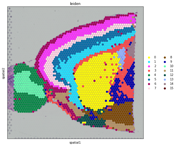
../_images/tutorials_10x_Visium_mouse_brain_15_1.png

We also visualize the inferred spatial domains in spatial coordinates.

[10]:

fig, axs = plt.subplots(figsize=(9, 7))

sc.pl.spatial(
    adata,
    img_key="hires",
    color="leiden",
    size=1.5,
    palette=sc.pl.palettes.default_102,
    legend_loc='right margin',
    show=False,
    ax=axs,
)

plt.tight_layout()

../_images/tutorials_10x_Visium_mouse_brain_17_0.png

Spatial domain annotation#

After spatial domain identification, we compute the differentially expressed (DE) genes of each domain for annotation.

[11]:

sc.tl.rank_genes_groups(adata, groupby='leiden', method='t-test')

[12]:

marker_genes = pd.DataFrame(adata.uns['rank_genes_groups']['names']).iloc[:10,:]
marker_genes

[12]:

	0	1	2	3	4	5	6	7	8	9	10	11	12	13	14	15
0	Ppp1r1b	3110035E14Rik	Camk2n1	Plp1	Calb2	1110008P14Rik	Ptgds	Stx1a	Zcchc12	Mobp	Gng4	Nptxr	Tac1	Ttr	Neurod6	Scarf1
1	Gpr88	Slc17a7	Camk2a	Mobp	Doc2g	Scn1b	Myoc	Nrn1	Nap1l5	Mbp	Gpsm1	Olfm1	Ppp1r1b	Enpp2	Camk2a	1700102H20Rik
2	Pde10a	Ttc9b	Lamp5	Mbp	Fabp7	Cck	Mgp	Camk2n1	Bc1	Plp1	Pcbp3	Ttc9b	Rgs9	1500015O10Rik	Cabp7	Rin3
3	Rgs9	Nptx1	Cck	Mal	Slc6a11	Slc17a7	Gjb2	Slc17a7	Gaa	Trf	Synpr	Slc17a7	Gad2	Cd9	Nsmf	Zap70
4	Penk	Ncald	Nptxr	Trf	Cdhr1	Vsnl1	Aebp1	Cck	Nrsn2	Agt	Meis2	Ndrg3	Gpr88	Igfbp2	Shisa6	Slc15a3
5	Pde1b	Efhd2	Nrgn	Cldn11	Csdc2	Snap25	Col1a2	Nrgn	Ly6h	Mag	Pbx3	Stmn1	Adcy5	Kl	Neurod2	Map3k14
6	Scn4b	Olfm1	Olfm1	Mag	Th	Cplx1	Aldh1a2	Lingo1	Tmem130	Plekhb1	Ptpro	Lmo3	Gng7	Fxyd1	Hpca	Tep1
7	Adcy5	Tbr1	Enc1	Cnp	Nmb	3110035E14Rik	Atp1a2	Olfm1	Ndn	Mal	Cpne4	Chgb	Pde10a	Lbp	Cck	AU021092
8	Rasd2	Stmn1	Lingo1	Plekhb1	Gng4	Adcy1	Fmod	Nptxr	Gap43	Pvalb	Ablim3	Syp	Pcp4l1	Trf	Cnih2	Bmpr1b
9	Gng7	Cck	Atp1a1	Bcas1	Shisa8	Stmn1	Ogn	Nrsn1	Resp18	Sparc	Pbx1	Stmn2	Inf2	Folr1	Prkca	Znhit6

Then, we annotated these spatial domains accroding to their marker genes and spatial locations (reference: Allen Brain Reference Atlases).

[13]:

cluster2annotation = {
     '0': 'Striatum',
     '1': 'Cortical layer6',
     '2': 'Cortical layer2/3',
     '3': 'Fiber tracts',
     '4': 'Olfactory bulb(outer)',
     '5': 'Cortical layer5',
     '6': 'Cortical layer1',
     '7': 'Cortical layer4',
     '8': 'Hypothalamus',
     '9': 'Thalamus',
     '10': 'Olfactory bulb(inner)',
     '11': 'Subplate',
     '12': 'Striatum',
     '13': 'Choroid plexus',
     '14': 'Hippocampus',
     '15': 'Others',
}

[14]:

adata.obs['annotation'] = adata.obs['leiden'].map(cluster2annotation).astype('category')

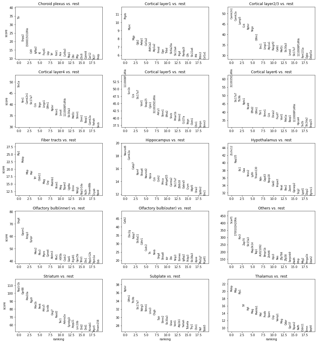
Spatial domain DE genes#

Lastly, we compute the differentially expressed (DE) genes of each annotated spatial domain for visualization.

[15]:

sc.tl.rank_genes_groups(adata, groupby='annotation', method='t-test')

[16]:

sc.pl.rank_genes_groups(adata, n_genes=20, ncols=3, sharey=False)

../_images/tutorials_10x_Visium_mouse_brain_26_0.png

[17]:

DE_genes = pd.DataFrame(adata.uns['rank_genes_groups']['names']).iloc[:10,:]
DE_genes

[17]:

	Choroid plexus	Cortical layer1	Cortical layer2/3	Cortical layer4	Cortical layer5	Cortical layer6	Fiber tracts	Hippocampus	Hypothalamus	Olfactory bulb(inner)	Olfactory bulb(outer)	Others	Striatum	Subplate	Thalamus
0	Ttr	Ptgds	Camk2n1	Stx1a	1110008P14Rik	3110035E14Rik	Plp1	Neurod6	Zcchc12	Gng4	Calb2	Scarf1	Ppp1r1b	Nptxr	Mobp
1	Enpp2	Myoc	Camk2a	Nrn1	Scn1b	Slc17a7	Mobp	Camk2a	Nap1l5	Gpsm1	Doc2g	1700102H20Rik	Gpr88	Olfm1	Mbp
2	1500015O10Rik	Mgp	Lamp5	Camk2n1	Cck	Ttc9b	Mbp	Cabp7	Bc1	Pcbp3	Fabp7	Rin3	Pde10a	Ttc9b	Plp1
3	Cd9	Gjb2	Cck	Slc17a7	Slc17a7	Nptx1	Mal	Nsmf	Gaa	Synpr	Slc6a11	Zap70	Rgs9	Slc17a7	Trf
4	Igfbp2	Aebp1	Nptxr	Cck	Vsnl1	Ncald	Trf	Shisa6	Nrsn2	Meis2	Cdhr1	Slc15a3	Pde1b	Ndrg3	Agt
5	Kl	Col1a2	Nrgn	Nrgn	Snap25	Efhd2	Cldn11	Neurod2	Ly6h	Pbx3	Csdc2	Map3k14	Penk	Stmn1	Mag
6	Fxyd1	Aldh1a2	Olfm1	Lingo1	Cplx1	Olfm1	Mag	Hpca	Tmem130	Ptpro	Th	Tep1	Adcy5	Lmo3	Plekhb1
7	Lbp	Atp1a2	Enc1	Olfm1	3110035E14Rik	Tbr1	Cnp	Cck	Ndn	Cpne4	Nmb	AU021092	Scn4b	Chgb	Mal
8	Trf	Fmod	Lingo1	Nptxr	Adcy1	Stmn1	Plekhb1	Cnih2	Gap43	Ablim3	Gng4	Bmpr1b	Gng7	Syp	Pvalb
9	Folr1	Ogn	Atp1a1	Nrsn1	Stmn1	Cck	Bcas1	Prkca	Resp18	Pbx1	Shisa8	Znhit6	Rasd2	Stmn2	Sparc

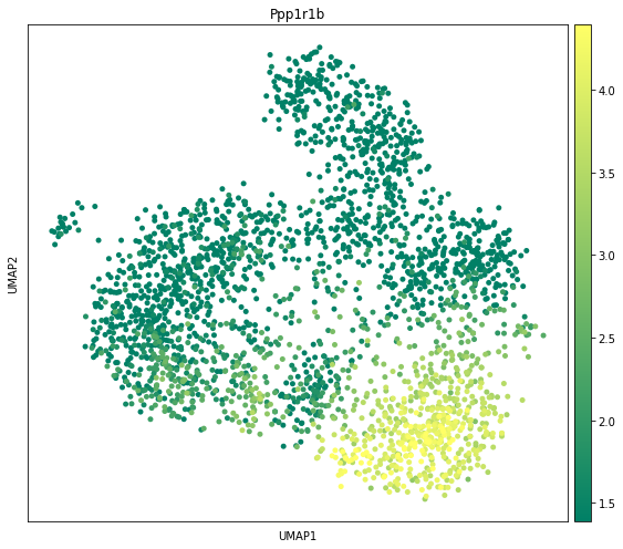
Now, we focus on a specific annotated spatial domain, here Striatum for demonstration.

We visualize the expression levels of the first-ranked DE gene of Striatum in UMAP space.

[18]:

fig, axs = plt.subplots(figsize=(8, 7))

sc.pl.umap(
    adata,
    color=DE_genes.iloc[0,12],
    size=100,
    cmap='summer',
    vmin='p50',
    vmax='p99',
    show=False,
    ax=axs,
)

plt.tight_layout()

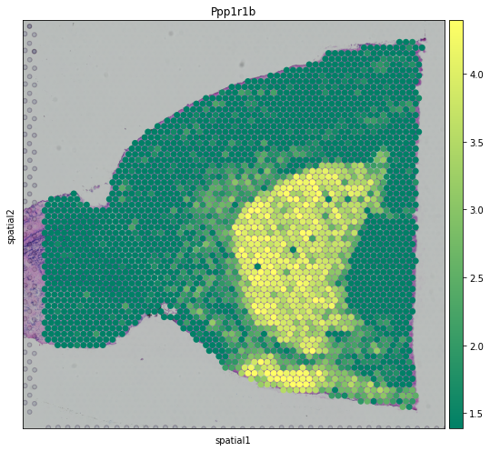
../_images/tutorials_10x_Visium_mouse_brain_29_0.png

We also visualize the expression levels of the first-ranked DE gene of Striatum in spatial coordinates.

[19]:

fig, axs = plt.subplots(figsize=(8, 7))

sc.pl.spatial(
    adata,
    img_key='hires',
    color=DE_genes.iloc[0,12],
    size=1.5,
    cmap='summer',
    vmin='p50',
    vmax='p99',
    show=False,
    ax=axs,
)

plt.tight_layout()

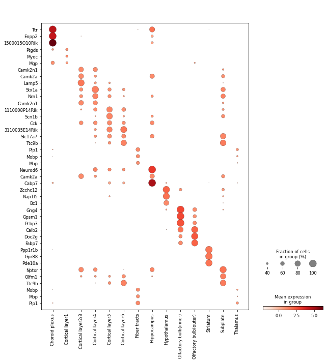
../_images/tutorials_10x_Visium_mouse_brain_31_0.png

Then, we scale the data and visualize the expression pattern of top 3 DE genes of each annotated spatial domain.

[20]:

sc.pp.scale(adata)

[21]:

fig, axs = plt.subplots(figsize=(9, 10))

sc.pl.dotplot(
    adata[adata.obs['annotation'] != 'Others', :],
    var_names=DE_genes.drop('Others', axis=1).iloc[0:3, :].to_numpy().T.reshape(-1),
    groupby='annotation',
    expression_cutoff=1,
    dot_min=0.25,
    swap_axes=True,
    show=False,
    ax=axs,
)

plt.tight_layout()

../_images/tutorials_10x_Visium_mouse_brain_34_0.png