Denoising and meta genes analysis of 10x Visium human breast cancer slice#

In this tutorial, we demonstrate SpaSRL on the gene expression denoising and functional meta genes analysis of 10x Visium Human Breast Cancer (Block A Section 1) slice including

Gene expression denoising
Functional meta genes

The dataset is available at 10x genomics website (Spatial Gene Expression >> Visium Demonstration (v1 Chemistry) >> Space Ranger 1.0.0 >> Human Breast Cancer (Block A Section 1)).

[1]:

import numpy as np
import pandas as pd
import scanpy as sc
import matplotlib.pyplot as plt
import SpaSRL

%matplotlib inline

Data loading and preprocessing#

We load the dataset after spatially aware self-representation learning in previous tutorial.

[2]:

adata = sc.read_h5ad('./data/BC_results.h5ad')
adata

[2]:

AnnData object with n_obs × n_vars = 3813 × 33538
    obs: 'in_tissue', 'array_row', 'array_col', 'leiden', 'leiden_refined', 'annotation'
    var: 'gene_ids', 'feature_types', 'genome', 'highly_variable', 'highly_variable_rank', 'means', 'variances', 'variances_norm'
    uns: 'annotation_colors', 'hvg', 'leiden', 'leiden_refined_colors', 'pca', 'rank_genes_groups', 'representation', 'spatial', 'spatial_enhancement'
    obsm: 'spatial'
    varm: 'PCs'
    layers: 'counts', 'log1p'
    obsp: 'representation'

Gene expression denoising#

We perform gene expression denoising using representation matrix.

[3]:

SpaSRL.expression_denoising(adata)

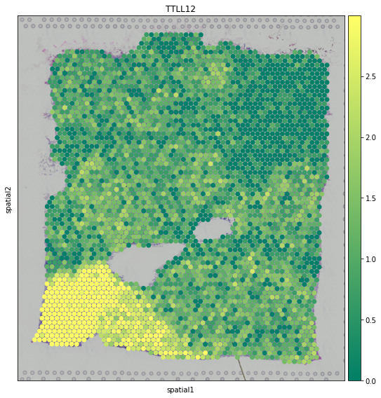
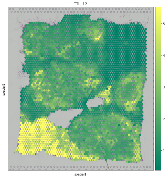
We show the spatial expression pattern of TTLL12 (differentially expressed in tumor domain) before and after denoising.

[4]:

fig, axs = plt.subplots(figsize=(8, 8))

sc.pl.spatial(
    adata,
    img_key='hires',
    color='TTLL12',
    layer='log1p',
    size=1.5,
    cmap='summer',
    vmin='p10',
    vmax='p95',
    show=False,
    ax=axs,
)

plt.tight_layout()

../_images/tutorials_denoising_and_meta_genes_10_0.png

[5]:

fig, axs = plt.subplots(figsize=(8, 8))

sc.pl.spatial(
    adata,
    img_key='hires',
    color='TTLL12',
    size=1.5,
    cmap='summer',
    vmin='p10',
    vmax='p95',
    show=False,
    ax=axs,
)

plt.tight_layout()

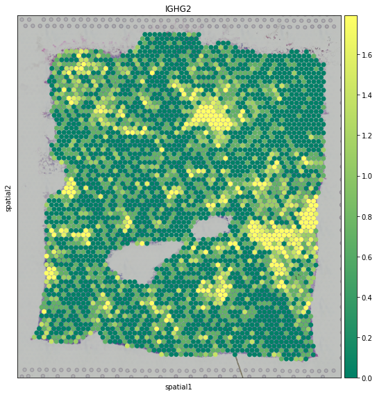
../_images/tutorials_denoising_and_meta_genes_11_0.png

We also show the spatial expression pattern of IGHG2 (differentially expressed in immune domain) before and after denoising.

[6]:

fig, axs = plt.subplots(figsize=(8, 8))

sc.pl.spatial(
    adata,
    img_key='hires',
    color='IGHG2',
    layer='log1p',
    size=1.5,
    cmap='summer',
    vmin='p10',
    vmax='p95',
    show=False,
    ax=axs,
)

plt.tight_layout()

../_images/tutorials_denoising_and_meta_genes_13_0.png

[7]:

fig, axs = plt.subplots(figsize=(8, 8))

sc.pl.spatial(
    adata,
    img_key='hires',
    color='IGHG2',
    size=1.5,
    cmap='summer',
    vmin='p10',
    vmax='p95',
    show=False,
    ax=axs,
)

plt.tight_layout()

../_images/tutorials_denoising_and_meta_genes_14_0.png

Functional meta genes#

We compute functional meta gene score matrix using discriminant matrix.

[8]:

SpaSRL.get_meta_genes(adata)

We create a new object adata_meta_genes using the meta gene score matrix for visualization.

[9]:

adata_meta_genes = sc.AnnData(adata.obsm['meta_genes'])
adata_meta_genes.obs = adata.obs.copy()
adata_meta_genes.obsm = adata.obsm.copy()
adata_meta_genes.uns['spatial'] = adata.uns['spatial'].copy()
sc.pp.scale(adata_meta_genes)

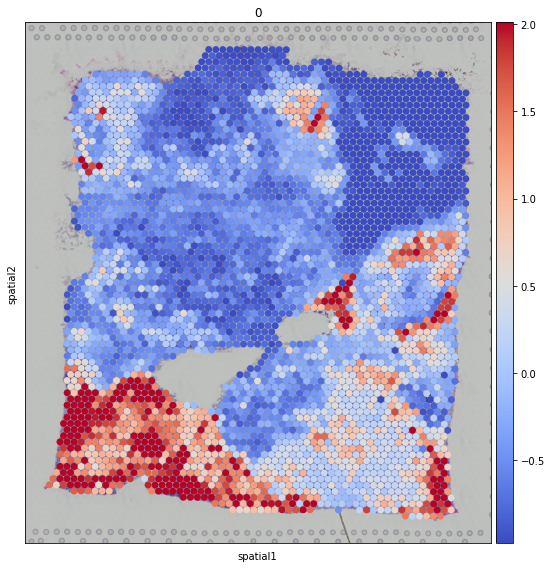
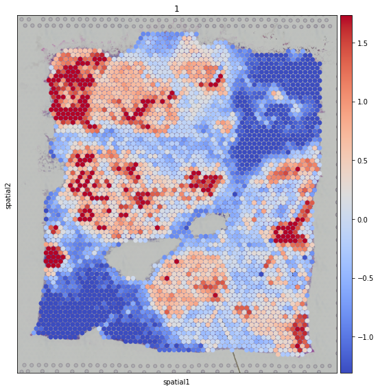
We show the spatial meta gene score pattern of 3 representative meta genes.

[10]:

fig, axs = plt.subplots(figsize=(8, 8))

sc.pl.spatial(
    adata_meta_genes,
    img_key='hires',
    color='0',
    size=1.5,
    cmap='coolwarm',
    vmin='p10',
    vmax='p95',
    show=False,
    ax=axs,
)

plt.tight_layout()

../_images/tutorials_denoising_and_meta_genes_21_0.png

[11]:

fig, axs = plt.subplots(figsize=(8, 8))

sc.pl.spatial(
    adata_meta_genes,
    img_key='hires',
    color='1',
    size=1.5,
    cmap='coolwarm',
    vmin='p10',
    vmax='p95',
    show=False,
    ax=axs,
)

plt.tight_layout()

../_images/tutorials_denoising_and_meta_genes_22_0.png

[12]:

fig, axs = plt.subplots(figsize=(8, 8))

sc.pl.spatial(
    adata_meta_genes,
    img_key='hires',
    color='2',
    size=1.5,
    cmap='coolwarm',
    vmin='p10',
    vmax='p95',
    show=False,
    ax=axs,
)

plt.tight_layout()

../_images/tutorials_denoising_and_meta_genes_23_0.png